Estimating System Parameters
First, I needed to set up the model of the system (i.e. the dynamics of the robot). We can model the robot as a second order system (with respect to position) that is governed by the following state space equation:
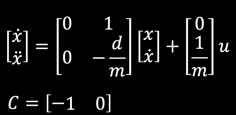
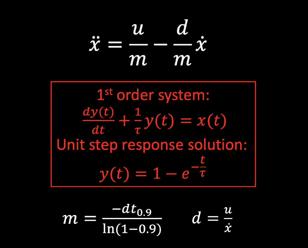
To find the system parameters m (mass) and d (drag coefficient), we consider the first order dynamics of the robot's velocity. Since we know the unit step response solution of a first order system, we can infer the system parameters from the step response rather easily.
I obtained the step response of my robot by inputting a constant PWM signal of 110.
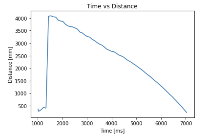
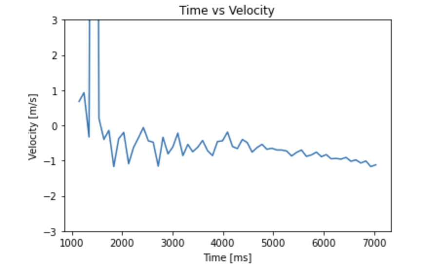
The steady state velocity from the step input was 1.12 m/s. The time taken to reach 90 percent of this steady state value was 6.445 seconds. For the sake of simplicity, I assumed unit step input (i.e. 110 PWM = 1 unit input) to calculate m and d. This just means that I will have to normalize the input vector u by 110 later. d was calculated to be 0.0008928571429 and m was calculated to be 0.00249913208. Now that I have values for m and d, I can predict the future states of the system given the input u. The advantage of this is that I can infer the robot's state (i.e. position and velocity) even without ToF sensor readings. So I will no longer have to rely on the sensor to determine the position of the robot. This effectively increases the frequency of the control loop.
Simulating the Kalman filter on Lab 6 Data
Because the system (robot) works in discrete time, I first had to discretize the system matrices A and B. I used to equations given in lecture to do this. The equations are:
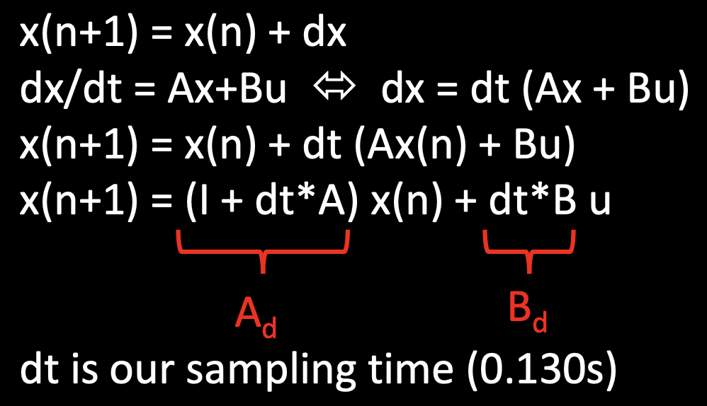
The sampling time used was 100 ms because that's approximately how long it takes for the ToF sensor to make a measurement. Then I had to determine a value for the measurement noise (sigma z). An easy way to do this is to leave the robot still and see how much noise there is in the sensor readings. There was about a 20 mm fluctuation in the sensor's measurements so I used a value of 20 mm for sigma z. Then I had to figure out how much trust to put in the model of the system that we developed in the previous section. The matrix containing this information is called the process noise (sigma u). I just used the values given in lecture for the process noise (27.7 mm for position and 27.7 mm/s for velocity). Finally, I could input these values into the Kalman filter. The code for the Kalman filter is given below:
Then I simulated the Kalman filter on the data from lab 6. Here is the code that simulates the Kalman filter on this data:
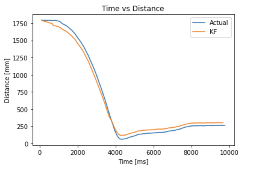
'distance' is an array containing the distance sensor data from lab 6. 'time' is the time stamp array for these distance sensor readings.'u' is an array containing the motor input that was given to the robot in lab 6. Given the input 'u' and the system matrices, the model can predict the future states of the system based on what input you give it. The Kalman filter "fuses" the sensor data and the distance predicted by the model to give a more accurate estimation of the robot's distance from the wall. Here is the result of running the Kalman filter on the lab 6 data:
Using extrapolation to increase sampling rate
Implmenting the Kalman filter on my real robot proved to be challenging. Therefore, I instead decided to increase the sampling rate (i.e. frequency of the control loop) by using extrapolation. By extrapolation, I mean using past ToF data to predict future position of the robot. The way I approached this was to take the last two ToF data to calculate a velocity value. If the sensor data is ready, the robot just uses the sensor data. But if sensor data is not ready, the robot uses the velocity value to propate the robot's position in time. Since each loop takes about 10 ms, I take the current distance and add velocity•10ms to get the next distance value. The code for extrapolation is given below:
Here is a video of the robot running this code to execute PID position control:
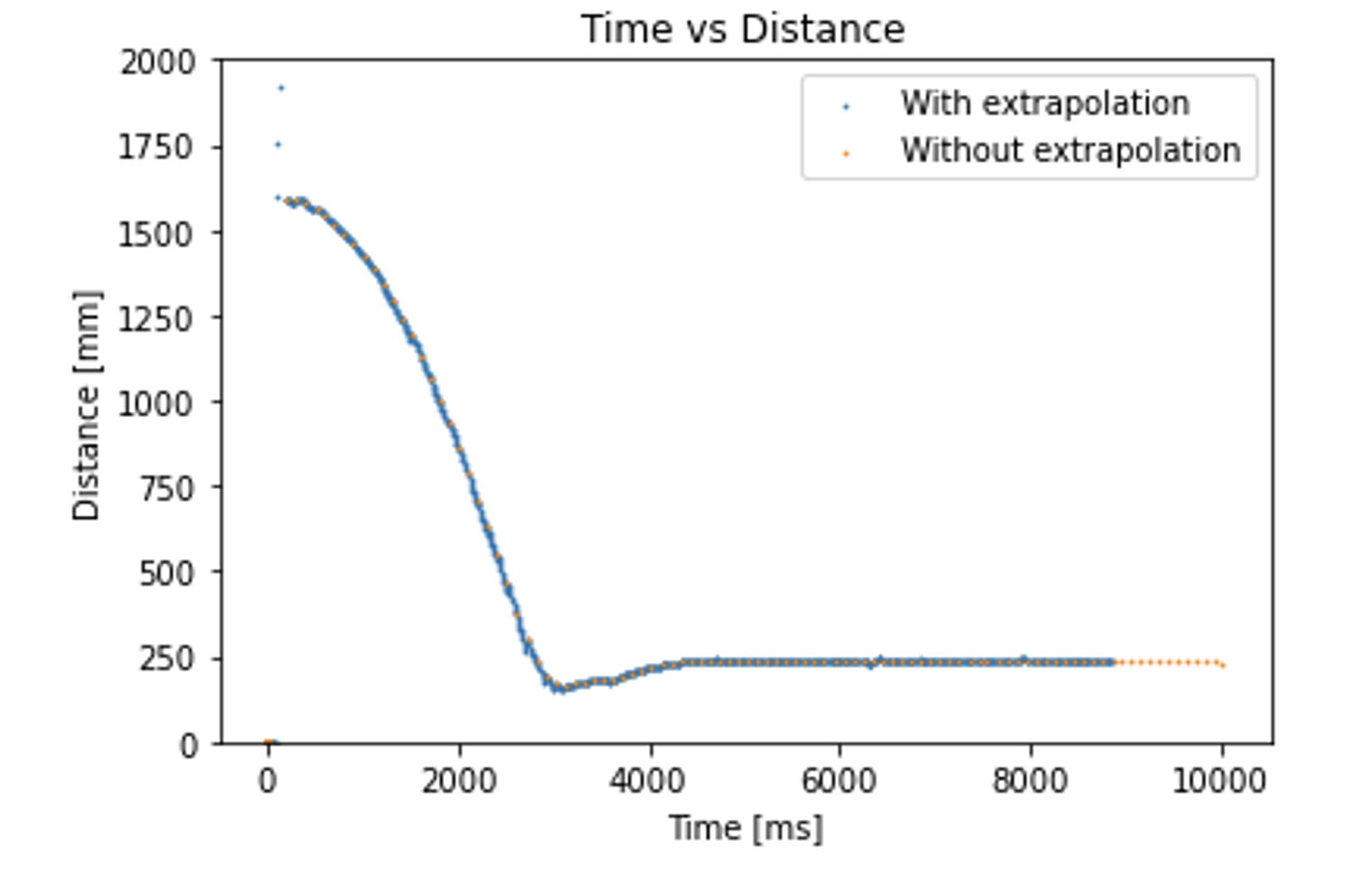
Here is a plot of the time vs. distance data collected by the robot:
Here is the same plot but zoomed into the first couple of seconds of the task:
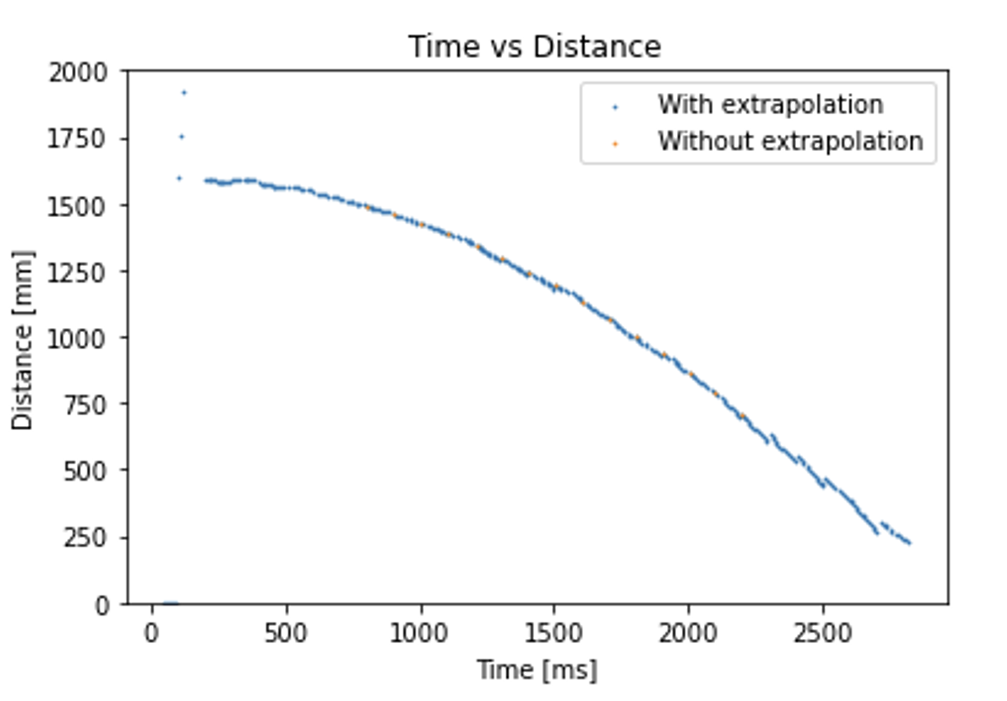
You can see that the orange dots (data without extrapolation) are much more sparse than the blue dots (data with extrapolation). This shows that the extrapolation code successfully increased the sampling rate. Also, the blue dots do not stray off much from the trend of the sensor readings (orange dots) so the extrapolation seems to be reasonably accurate as well. According to the recorded time stamps, it takes about 10 milliseconds on average in order to execute the loop once. So given that it takes about 100 ms for the ToF sensor to make a measurement, this extrapolation method effectively increases the sampling rate about tenfold.